Perceptron and Generalized Linear Model

Perceptron

Perceptron algorithm is not something that is widely used in practice. We study it mostly for historical reasons. And also it’s nice and simple, and easy to analyze.

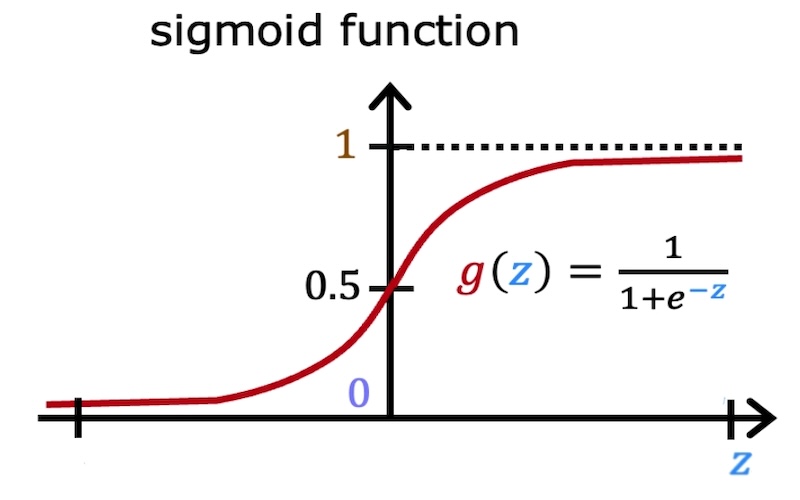
As you know, Logistic Regression uses the Sigmoid Function. Which essentially squeezes the entire real line, from $-\infty$ to $+\infty$, between 0 and 1, and the 0 and 1 kind of represent the probability of the output being 1.

The Perceptron algorithm uses a somewhat similar but different, and you can think of that as the hard version of sigmoid function. Which is that it outputs either 0 or 1, and it’s not going to output any value in between.

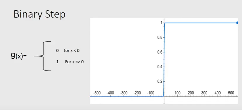
And this leads to the hypothesis function, which defines the output as follows:

And as you know, for logistic regression, the hypothesis function is defined as follows, based on the sigmoid function:

So , the update rule for both logistic regression and perceptron is the same, and it’s defined as follows:

They look the same, except the hypothesis function is different.

As you know, this quantity, $y^{(i)}-h_\theta(x^{(i)})$ in the update rule, is a scalar. It’s the difference between the actual output $y$, which can be either 0 or 1, and the hypothesis function $h_\theta(x^{(i)})$ which is either 0 or 1. So, when the algorithm makes a prediction, that quantity will either be 0 or 1, as follows:

• $0 \rightarrow \quad \text{algorithm got it right}$
• $+1 \rightarrow \quad \text{algorithm got it wrong and} \quad y^{(i)}=1$
• $-1 \rightarrow \quad \text{algorithm got it wrong and} \quad y^{(i)}=0$

Imaging there are two classes, boxes and circles, and you want to learn an algorithm to separate these two classes. And what the algorithm has learned so far is a $\theta$ that represents the blue color decision boundary, which represent $\theta^T x = 0$. And anything above is $\theta^T x > 0$ and anything below is $\theta^T x < 0$.

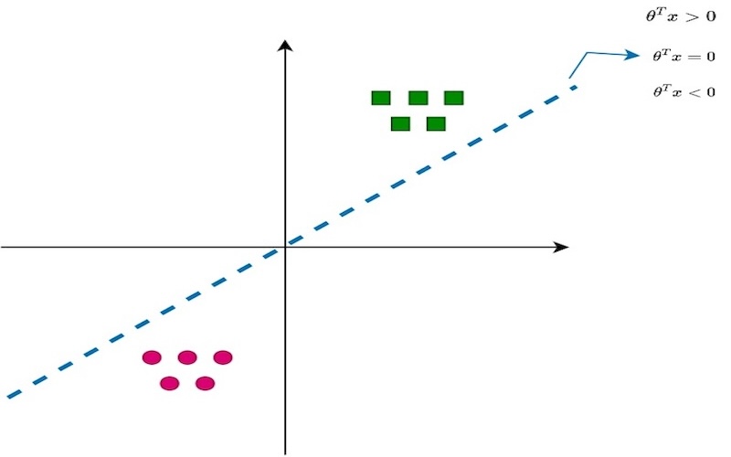
And let’s say the algorithm is learning one example at a time, and a new example comes in. and the new example happens to be a box, which is colored blue. And the algorithms is mis-classified it now. The blue line which separating boundary, if the vector equivalent of that would be a vector that’s normal to the line, which is the vector $\theta$ and shown in red arrow. And the new example is the new $x$. Let’s say the boxes are class 1 and the circles are class 0. And what the update rule does is, sets $\theta$ to be $\theta + \alpha x$. So the new $\theta$ is now shown in green arrow. It’s the new vector and updated value of $\theta$. And the separating hyperplane corresponding to that is shown in green color.

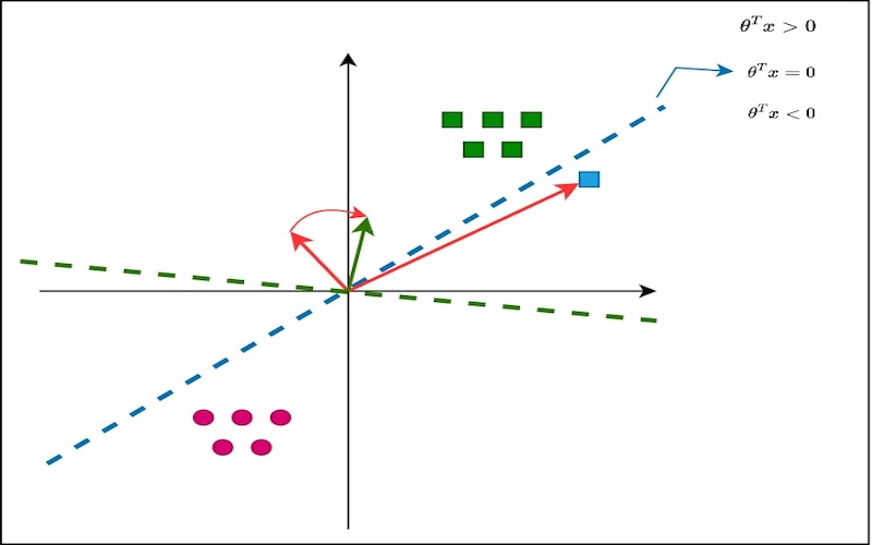
So, it updated the decision boundary such that new example is now included in the positive class. And the idea here is that:

The reason is when two vectors are similar, the dot product is positive, if the angle is less than $r = 90^\circ$, and when they are not similar, the dot product is negative, if the angle is greater than $r = 90^\circ$.

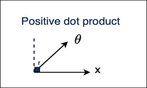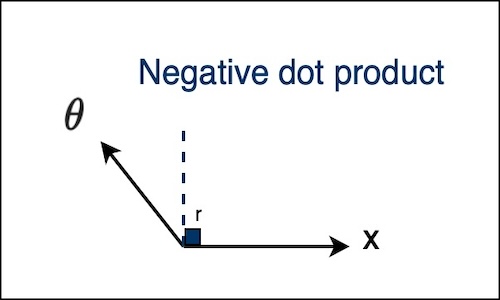So, this is essentially means that as $\theta$ is rotating, the decision boundary is kind of perpendicular to the vector $\theta$. And you wanna get all the positive examples on one side of the decision boundary.

And what’s the most naive way of taking $\theta$ and given $x$ try to make $\theta$ more kind of closer to $x$? A simple thing is to just add a component of $x$ in that direction and kind of make $\theta$. And this is a very common technique used in lots of algorithms, where essentially if you add a vector to another vector, you make the second one kind of closer to the first one.

So, this is the Perceptron algorithm. You go example by example in an online manner, and if the example is already classified, you do nothing, you got a 0 in the quantity $y^{(i)}-h_\theta{(x^{(i)})}$ in the update rule. And if it is misclassified, you either add the example itself to you $\theta$ or you subtract it from $\theta$, depending on the class of the vector.

Why don’t we use them in practice? You kinda have a geometrical feel of what’s happening with the hyperplane but it doesn’t really give you a probabilistic interpretation of what’s happening. The perceptron was pretty famous in 1950’s and 1960’s, where people thought this is a good model of how brain works. And it was Marvin Minsky¹, who wrote a paper saying the perceptron is kind of limited because it could never classify the XOR function and example points like that. So do something as simple as this, and kind of people lost interest in it. And this paper was very influential, and it kind of killed the interest in neural networks for a long time. And in fact, what we see in logistic regression is, it’s like a soft version of the perceptron itself in a way.

It’s up to you when you wanna stop training, a common thing is to just decrease the learning rate $\alpha$ over time, until you stop making changes.

Exponential Family

Exponential family is a class of probability distributions, which are somewhat nice mathematically. They’re also very closely related to GLMs (Generalized Linear Models) which we’ll see later.

Probability Density Function (PDF)

For a discrete distribution, then it would be the probability mass function (PMF). Whose PDF can be written as follows:

Where:

• $y$ is the data
  And there is a reason why we call it $y$ and not $x$. And that’s because we’re gonna use exponential families to model the output of your data, in a supervised learning setting. For most of our examples is going to be a scalar.
• $\eta$ is the natural parameter. Can be a vector, except maybe in softmax this would be a scalar. Has to match the dimension of $T(y)$.
• $T(y)$ is the sufficient statistic. And because all the distributions that we’re going be seen in this post, $T(y) = y$. Has to match the dimension of $\eta$.
• $b(y)$ is the base measure. It is scalar.
• $a(\eta)$ is the log-partition function. It is scalar.

Note that $T(y)$ and $b(y)$ are functions of only $y$. These functions cannot involve $\eta$. And $a(\eta)$ has to be a function of only $\eta$ and constants.

And the reason why $a(\eta)$ is called the log-partition function is pretty easy to see, because this can be written as follow:

And these two are exactly the same. You can think of this as a normalizing constant of the distribution such that the whole thing integrates to 1. So the partition function is a technical term to indicate the normalizing constant of probability distributions.

For any choice of $T(y)$, $b(y)$, and $a(\eta)$, that can be your choice completely, as long as the expression integrates to 1, you have a family in the exponential family.

What does that mean is for a specific choice of $T(y)$, $b(y)$, and $a(\eta)$, the $\mathcal{P}(y; \eta)$ will be equal to PDF of Gaussian, and for that choices, you got a family of Gaussian distribution. Such that for any value of the parameter, you get a member of the Gaussian family.

Usage of Exponential Families

Depending on the kind of data that you have, you can choose any member of the exponential family, as parameterized by $\eta$.

• If you have real value data, it can take any value between 0 and $\infty$, then, you use a Gaussian distribution.
• If you have binary data, it can only take two values, 0 or 1, then, you use a Bernoulli distribution.
• If you have count data, that means just non-negative integers, then, you use a Poisson distribution.
• If you have positive real value integers, like the volume of some object or a time to an event which that you are only predicting into the future, then, you can use a Gamma or Exponential distribution.
• You can also have probability distributions over probability distributions, like Beta, Dirichlet, these mostly show up in Bayesian Machine Learning or Bayesian Statistics.

Bernoulli Distribution

Is a distribution we use to model binary data. And below is the PDF of the Bernoulli distribution:

Where:

• $\phi$ is the probability of the event happening or not.

This pattern is like a way of programmatic if, else statement in math. So whenever $y=1$, the second term cancels out, and the answer would be $\phi$, and whenever $y=0$, the first term cancels out, and the answer is $(1-\phi)$.

Now, let’s see how this can be written in the exponential family form.

Now, if start doing pattern matching from this and the exponential family form, we can see that:

• $b(y) = 1$
• $T(y) = y$
• $\eta = \log(\frac{\phi}{1-\phi}) \rightarrow \phi = \frac{1}{1 + e^{-\eta}} \rightarrow \text{This like the sigmoid function}$
• $a(\eta) = -\log(1-\phi) \rightarrow -\log(1-\frac{1}{1+e^{-\eta}}) = \log(1+e^\eta)$

First with start with a log partition function that is parameterized by the canonical parameters, and we use the link between the canonical parameters and the natural parameters, invert it, and then we get the natural parameters.

So, this kind of verifies that the Bernoulli distribution is a member of the exponential family.

Gaussian Distribution (with fixed variance)

Gaussian distribution has two parameters, the mean and the variance. In this post we’re gonna assume a constant variance, you can also consider Gaussian with where the variance is also a variable.

We are going to assume that the variance is equal to 1. So this gives the PDF of a Gaussian to look like this:

Now, if start doing pattern matching from this and the exponential family form, we can see that:

• $b(y) = \frac{1}{\sqrt{2\pi}} \exp(-\frac{y^2}{2})$
• $T(y) = y$
• $\eta = \mu$
• $a(\eta) = \frac{\mu^2}{2}$

Same as the Bernoulli distribution, we start with a log partition function that is parameterized by the canonical parameters, and we use the link between the canonical parameters and the natural parameters, invert it, and then we get the natural parameters.

So, this kind of verifies that the Gaussian distribution is a member of the exponential family.

Properties of Exponential Families

So these are exponential families. The reason why we use exponential families is because it has some nice mathematical properties.

• a

  • MLE with respect to $\eta$ $\Rightarrow$ concave.
    If we perform maximum likelihood estimation (MLE) on the exponential family, when the exponential family is parameterized in the natural parameters, then the optimization problem is concave.

  • NLL $\Rightarrow$ convex.
    Negative log-likelihood, so take a log of the expression, negate it and in this case, is like the cost function equivalent of doing maximum likelihood. So, You’re just flipping the sign, instead of maximizing, you minimize the negative log-likelihood.

• b

  • $E[y; \eta] = \frac{\partial}{\partial\eta} a(\eta)$
    Each of the distribution, we start with $a(\eta)$, differentiate the log partition function with respect to $\eta$, and you get another function with respect to $\eta$. And this function is the mean of the distribution as parameterized by $\eta$.
    It was the first derivative.

• c

  • $Var[y; \eta] = \frac{\partial^2}{\partial\eta^2} a(\eta)$
    This is the variance of the distribution as parameterized by $\eta$. It was the second derivative.

In general for probability distribution to calculate the mean and variance, you need to integrate something, but over here we just need to differentiate, which is much easier operation.

Note that if it’s a multi-variate Gaussian, then this $\eta$ would be a vector, and the mean and variance would be a function of $\eta$. And this $\frac{\partial^2}{\partial\eta^2} a(\eta)$ would be a the Hessian matrix.

Generalized Linear Model (GLM)

GLM is somewhat like a natural extension of the exponential families to include covariates or input features in some way. So in the exponential families, we’re only dealing with the $y$, which in our case it’ll kind of map to the outputs. But we can actually build a lot of many powerful models by choosing an appropriate family in the exponential family, and kind of plugging it onto a linear model. So assumptions or design choices that are gonna take us from exponential families to GLMs are:

• (i)
  The most important assumption is that:
  
  $$ y \vert x; \theta \sim \text{Exponential Family}(\eta) $$
• (ii)
  The design choice that we are making is:
  
  $$ \eta = \theta^T x \qquad \theta \in \mathbb{R}^n , x \in \mathbb{R}^d $$
  So this is where your $x$ now comes into the picture.
  $n$ has nothing to do with anything in the exponential family, it’s purely, a dimensions of your data that you have, of the $x$ of your input.
  We make a design choice that $\eta$ will be $\theta^T x$.
• (iii)
  At test time, when we want an output for a new example $x$, the output will be:
  
  $$ E[y; \theta^T x] $$
  So, given an $x$, we get an exponential family distribution, and the mean of that distribution will be the prediction that we make for a given $x$. So what this essentially means is that:
  $$ h_\theta(x) = E[y \vert x; \theta] $$
  This is our hypothesis function. And what we do over here, if you plug in the exponential family, as Gaussian, then the hypothesis will be the same as the Gaussian hypothesis that we saw in linear regression.
  If we plug in a Bernoulli, then this will turn out to be the same hypothesis that we saw in logistic regression.

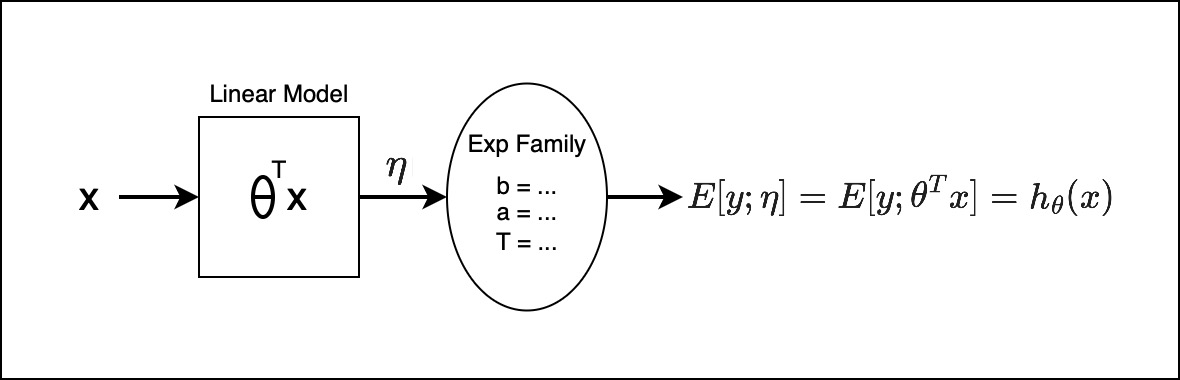
Let’s visualize this:

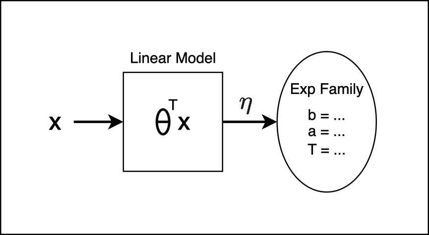
There is a model, in square box, and a distribution, in oval box, So, the model we are assuming it to be a linear model. Given $x$, there is a learnable parameter $\theta$, and $\theta^T x$ will give you a parameters $\eta$. Now the distribution is a member of the exponential family, and the parameter for this distribution is the output of the linear model.

And the exponential family we make, depending on the data that we have, whether it’s a classification problem or a regression problem or a time to vent problem. You would choose an appropriate $b$, $a$, and $T$, based on the distribution of your choice. So this entire thing, and from that, you get the:

And this is essentially out hypothesis function.

The question is, are we training $\theta$ to predict the parameter of exponential family distribution, whose mean is the prediction that we’re gonna make for $y$? That’s correct.

So this is what we do at test time. And during training time, how do we train this model? So in this model, the parameter that we are learning by doing gradient descent are these parameters: $\theta^T x$. So you’re not learning any parameters in the exponential family, we’re not learning $\mu$ or $\sigma^2$ or $\eta$. We’re learning $\theta$ that’s part of the model, and not part of the distribution. And the output of this will become the distributions parameter. It’s unfortunate that we use the word parameter for both, but it’s important to understand what is being learned during training phase and what’s not. So this parameter $\eta$ is the output of a function, its not a variable that we do gradient descent on.

So, during training, what we do is maximum likelihood. Maximize with respect to $\theta$:

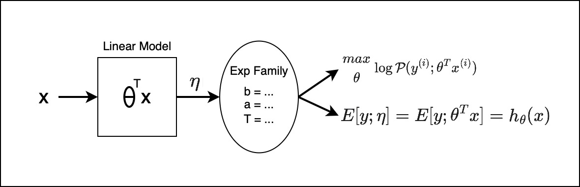
So, you’re doing gradient ascent on the log probability of $y$ where natural parameter was re-parameterized with the linear model. And we are doing gradient ascent byt taking gradients on $\theta$.

This is like a big picture of what’s happening with GLMs. And how they are an extension of exponential families. You re-parameterized the parameters with the linear model, and you get a GLM.

GLM Training

Let’s look at some more detail on what happens at train time. So, another kind of incidental benefit of using GLMs is that, at train time, we saw that you wanna do maximum likelihood using the log probability with respect to $\theta$. It turns out that, no matter what kind of GLM you’re doing, and which choice of distribution that you make, the learning update rule is the same:

And you can go straight to the update rule and do your learning. You plug in the appropriate $h_\theta(x)$, depending on the choice of distribution that you make and you can start learning, initialize you $\theta$ to some random values and you can start learning.

If you wanna do it for batch gradient descent, then you just sum over all you examples.

Newton method is probably the most common you would use with GLMs, and that again comes with the assumption that, dimensionality of your data is not extremely high. As long as the number of features is less than a few thousand, then you can use Newton’s method.

So that is the same update rule for any specific type of GLM based on the choice of distribution that you have. Whether you are modeling a classification problem or a regression problem, or a Poisson regression, the update rule is the the same.

Terminology

Some more terminology:

And the function that links the natural parameter to the mean of the distribution is called the Canonical Response Function.

Similarly, you can go from $\mu$ back to $\eta$ with the inverse of this:

We also, already saw that, $g(\eta)$ is also equal to the gradient of the log-partition function with respect to $\eta$.

3 Parameterizations

And it’s also helpful to make explicit the distinction between the three different kinds of parameterizations we have.

So we have:

• Model parameters $\rightarrow \theta$
• Natural parameters $\rightarrow \eta$
• Canonical parameters:
  • $\phi \rightarrow \text{Bernoulli}$
  • $\mu, \sigma^2 \rightarrow \text{Gaussian}$
  • $\lambda \rightarrow \text{Poisson}$

So, these are three different way we can parameterize, either the exponential family or the GLM. And whenever we learning a GLM, it is only this $\theta$ that we learn, that is the $\theta$ in the linear model.

And the connection between the natural parameter $\eta$ and the model parameter $\theta$ is linear. So:

And that is the design choice that we’re making. We choose to reparameterize $\eta$ by a linear model, linear in your data.

And between the natural parameter $\eta$ and the canonical parameters, you have:

Where $g$ is also the derivative of the log-partition function with respect to $\eta$.

It can get pretty confusing when you’re seeing this for the first time, because you have so many parameters that are being swapped around and getting reparameterized. There are three different ways in which we are parameterizing generalized linear models.

The model parameters $\theta$, the ones that we learn and the output of this is the natural parameter $\eta$ for the exponential family, and you can do some algebra manipulations and get the canonical parameters for the distribution that we are choosing, depending on the task where there’s classification or regression or something else.

Now, it’s actually pretty, you can see that, when you are doing logistic regression:

Because, here the choice of distribution is a Bernoulli, and the mean of a Bernoulli distribution is just $\phi$, in the canonical parameter space.

So the logistic function which when we introduced logistic regression, we just pulled out the logistic function out of thin air and say this is something that can squash $-\infty$ to $\infty$, between $0$ and $1$, seems like a good choice. But now we see that it is a natural outcome, it just pops out from that more elegant generalized linear model, where if you choose Bernoulli to be the distribution of your output, then the logistic regression just pops out naturally.

The choice of what distribution you are going to choose, is really dependent on the task that you have. So if your task is regression, where you want to output real valued numbers like price of the house or something, then you choose a distribution over the real numbers like a Gaussian. And if your task is classification, where your output is binary 0 or 1, you choose a distribution that models binary data like a Bernoulli. And if your task is count data, like modeling the number of visitors to a website which is like a count, then you choose a distribution that models count data like a Poisson distribution, because Poisson distribution is a distribution over integers.. So the task in a way influences you to pick the distribution, and most of the times that choice is pretty obvious.

So the task pretty much tells you what distribution you want to choose, and then you go through those machinery of figuring out what $h_\theta(x)$ is, and you plug in the formula and you have your learning rule.

Are GLMs used for classification, or are they used for regression? or are they used for something else? The answer really depends on what is the choice of distribution that you’re gonna choose. GLMs are just a general way to model data, and that data could be binary, or real value, and as long as you have a distribution that can model that kind of data and falls in the exponential family, it can be just plugged into a GLM and everything just works out nicely.

Assumptions of GLMs

Let’s start with Regression. We assume there is some $x$. To simplify, we’re drawing $x$ as one dimension, but it could be multi-dimensional. And there is $\theta$ and $\theta^T x$ would be some linear hyperplane and we assume that as the natural parameter $\eta$. And in case of regression, $\eta$ was also $\mu$. And then we are assuming that the $y$ for any given $x$, is distributed as a Gaussian with $\mu$ as the mean. So which means, for every possible $x$, you have the appropriate $\eta$, and with this as the mean, that is a Gaussian distribution. And note that we assume a variance of 1, so this is like a Gaussian with standard deviation or variance equal to 1. So for every possible $x$, there is a $y$ given $x$, which is parameterized by $\theta^T x$ as the mean.

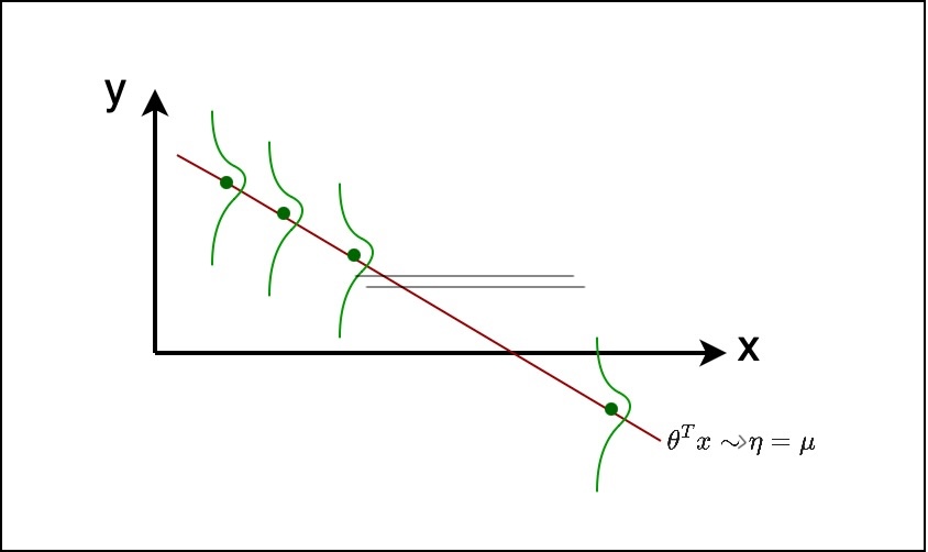
And, you assume that your data is generated from this process. So it means, you’re give $x$, you would have examples in your training set.

the assumption here is that, for every $x$, there is a Gaussian distribution that started from the mean over there, and from that Gaussian distribution, you sampled the value of $y$. You’re just sampling it from the distribution. So this is how your data is generated, and this is our assumption.

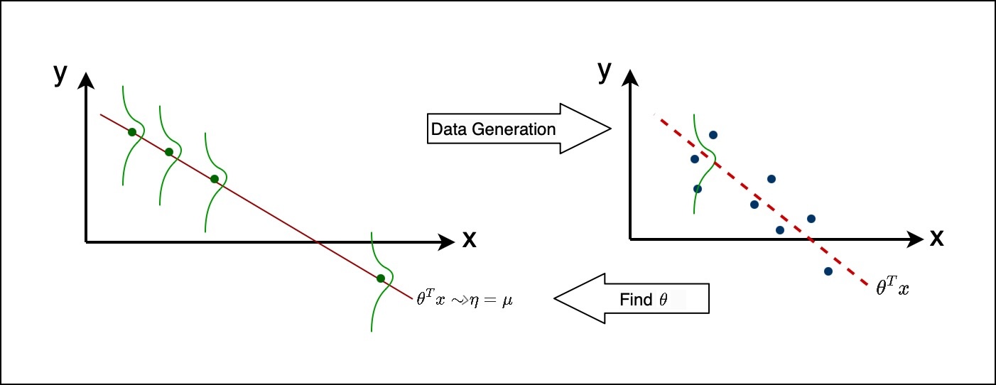
Now, based on these assumptions, what we are doing with the GLM is, we start with the data, we don’t know anything else. We make an assumption that there is some linear model from which the data was generated in that format, and we want to work backwards, to find $\theta$ that will give us that hyperplane line. So for different choice of $\theta$, we get a different line, we assume that if that line represents the $\mu$’s, or the means of the $y$’s for that particular $x$, from which it’s sampled from, we are trying to find a line, which will be like $\theta^T x$, from which those $y$’s are most likely to have sampled. That’s essentially what’s happening when you do maximum likelihood with the GLM.

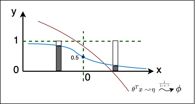
Similarly for classification, again let’s assume there’s an $x$, and some $\theta^T x$ which is equal to $\eta$. And from that $\eta$, we run this through the sigmoid function, $\frac{1}{1 + e^{-\eta}}$, to get $\phi$. So if those are the $\eta$s, for each $\eta$ we run it through the sigmoid and we get something like the blu line. And now, at any given choice of $x$, we have a probability distribution, in this case it’s a binary, so let’s assume probability of $y$ is the height to the sigmoid line. Every $x$ we have a different Bernoulli distribution, that’s obtained where, the probability of $y$ is the height to the sigmoid through the natural parameter.

And from that, you have a data generating distribution that would like the below:

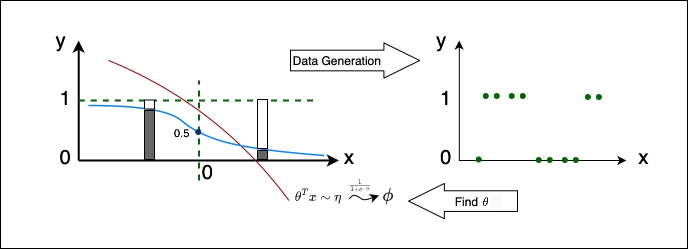
You have a few $x$s in your training set, and for those $x$s you figure out what your $y$ distribution is and sample from it. And now, given that data, we wanna work backward to find out, what $\theta$ was. What’s the $\theta$, that would have resulted in a sigmoid like curve from which those $y$s, were most likely to have been sampled. And figuring out that $y$ is essentially doing logistic regression.

Softmax Regression

In the lecture notes, Softmax Regression is explained as yet another member of the GLM family, however, in today’s lecture we’ll be taking a non-GLM approach and kind of see how softmax is essentially doing, what’s also called as cross entropy minimization. We’ll end up with the same formulas as equations. You can go through the GLM interpretation in the notes.

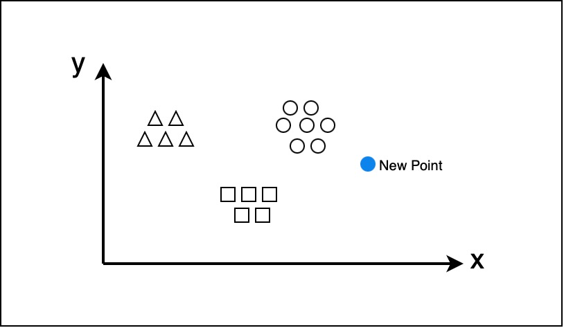
Here we talking about multiclass classification. So, let’s assume we have three classes of data, let’s call them circles, squares, and triangles. And the axises is $x_1$ and $x_2$, we’re just visualizing you input space and the output space $y$, is kind of implicit in the shape of this data.

In multiclass classification, our goal is to start from this data and learn a model that can given a new data point, make a prediction of whether this new point is a circle, square, or triangle. You’re just looking at three, because it’s easy to visualize but this can work over thousands of classes.

So, what we have is:

• $k$ is the number of classes
• $x^{(i)} \in \mathbb{R}^n$
• $$ \text{Label} \quad y^{(i)} = [\{1, 2\}^k] \quad \text{e.g.} \quad [0, 1, 0] $$
  So, the label $y$ is a one-hot vector, where it’s a vector which indicates which class the $x$ corresponds to. So each element in the vector, corresponds to one of the classes.
  So, for labels, we have a vector that’s filled with 0s, except with a 1, in one of the places.

And, the way we’re gonna think of softmax regression is that, each class, has it’s own set of parameters. So we have:

So in logistic regression, we had just one $\theta$, which would do a binary, yes versus no, in softmax we have one such vector of $\theta$ per class. So you could also optionally represent them as a matrix, $n$ by $k$ matrix.

So in softmax regression, it’s a generalization of logistic regression when you have a set of parameters per class.

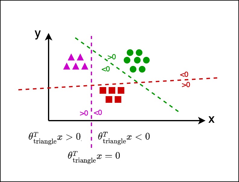
So, corresponding to each class of parameters that exists, there exists a line which represents, in our case, $\theta_\text{triangle}^T x = 0$, and anything to the left of that line, will be $\theta_\text{triangle}^T x > 0$, and anything to the right of that will be $\theta_\text{triangle}^T x < 0$.

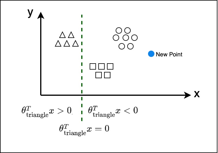
So, for the $\theta_\text{triangle}$ class, there is that line, which corresponds to #\theta^T x = 0$, anything to the left, will give you a value greater than zero, and anything to the right will give you a value less than zero.

Similarly, there is also a line for circles and squares.

So we have a different set of parameters per class which hopefully satisfies the property. And now out goal is to take these parameters and let’s see what happens when we have a new example.

So given an example $x$, we may get something that looks like this:

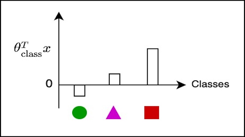
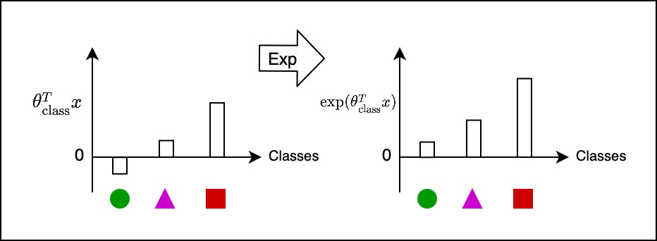
So, the space of $\theta_\text{class}^T x$, is also called the logic space, are real numbers, that is not a value between 0 and 1, that is between $-\infty$ and $+\infty$. And out goal is to get a probability distribution over the classes. And in order to do that, we perform a few steps. So we exponentiate the logic which would make everything positive.

Now we’ve got a set of positive numbers, and next we normalize that. By normalize, I mean, divide everything by the sum of all of them, and after normalization the sum of the heights will add up to 1. Once we do this operation, we get a probability distribution.

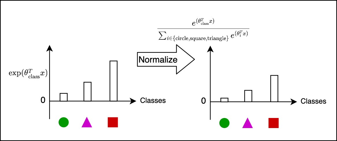
So, given a new point $x$, and we run through this pipeline, we get a probability output over the classes for which that example is most likely to belong to.

This is like out hypothesis function, $\hat{\mathcal{P}}(y)$. The output of the hypothesis function will output this probability distribution. In the other cases, the output of the hypothesis function, generally output a scalar or a probability, in this case, it’s output a probability distribution over all the classes.

For example, let’s say there is a new example, and it’s belongs to the triangle class, then the $\mathcal{P}(y)$, which also called the label, you can think of that as a probability distribution which is 1 over the correct class and 0 elsewhere. This is essentially representing the one-hot representation as a probability distribution.

Now, the goal or the learning approach that we’re going to do is in a way minimize the distance between these two distributions. We want to change the first distribution which is on the left, to look like the second distribution which is on the right.

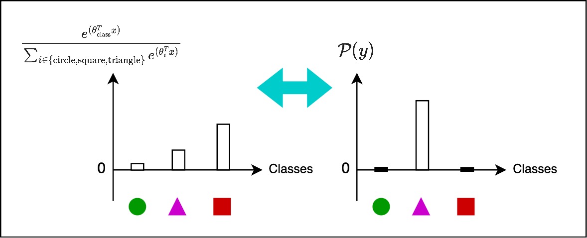
Technically, the term for that is minimize the cross entropy between the two distributions.

So, here we see that, $\mathcal{P}(y)$ will be 1 for just one of the classes, and 0 for the others, so let’s say in that example, the correct class for that new point is the triangle class, so this will essentially boil down to:

And we know that, the hypothesis is essentially this expression:

And you treat this as the loss and do gradient descent with respect to the parameters.