Locally Weighted Regression
Locally weighted regression is a way to modify linear regression and make it fit very non-linear functions, so you aren’t just fitting straight lines.
What if the data isn’t just fit well by straight line? how we can addressing out this problem? we wanna use the idea called locally weighted regression or locally weighted linear regression or LWR.
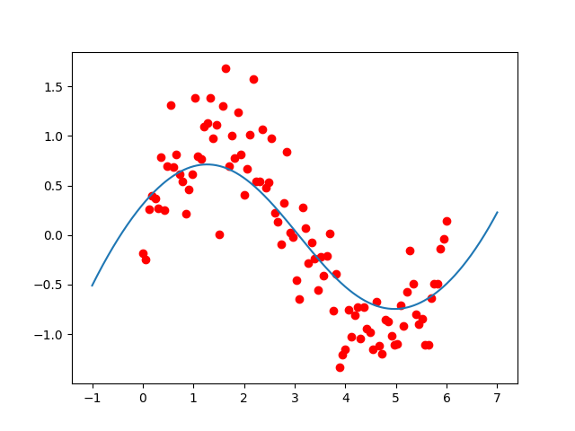
So it’s pretty clear what the shape of this data is, but how do you fit a curve that looks like this? It’s actually quite difficult to find features, is it $$ \sqrt x $$ or $$ \log x $$ or $$ x^\frac23 $$ and what is the set of features that lets you do this?
We’ll sidestep all those problems with an algorithm called locally weighted regression.
Parametric and Non-Parametric Learning Algorithms
To introduce a bit more machine learning terminology, in machine learning we sometimes distinguish between Parametric Learning Algorithms and Non-Parametric Learning Algorithms.
In a parametric learning algorithm, you fit some fixed set of parameters such as $$ \theta_i $$ to data, so linear regression as you saw in Linear Regression and Gradient Descent is a parametric learning algorithm. Because there’s a fixed set of parameters, the $$ \theta_i $$, so you fit to data and then you’re done.
Locally weighted regression is a non-parametric learning algorithm. And that means, the amount of data / parameters, you need to keep grows and in this case it grows linearly with the size of the data, the training set.
So, with the parametric learning algorithm, no matter how big your training set is, you fit the parameters $$ \theta_i $$, then you could erase a training set from your computer memory and make prediction just using the parameters $$ \theta_i $$.
But in non-parametric learning algorithm, the amount of stuff you need to keep around in computer memory, and you need to store around, grows linearly as a function of the training set size. So, this type of algorithm is may not be great if you have a really massive dataset, because you need to keep all of the data around, in computer memory or on disk just to make predictions.
One of effects of this, is that, it’ll be able to fit that data we saw before, quite well without you needing to fiddle manually with the features.
Now, for linear regression, if you want to evaluate $$ h $$ at a certain value of the input, and make a prediction, what you do is you fit $$ \theta $$, to minimize the cost function:
And then you return $$ \theta^T x $$. So you fit a straight line and then if you want to make a prediction at the value $$ x $$ you then return, say the $$ x^T $$.
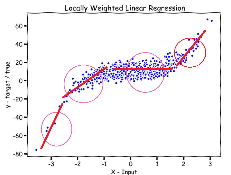
For locally weighted regression, you do something slightly different. Which is if we have a value of $$ x $$ and you want to make a prediction around that value, you look in a local neighborhood at the training examples close to that point where you want to make a prediction, and looking a little bit at further all examples, but really mainly focus on those example close to the value of $$ x $$, and you try to fit a straight line to those examples. Focusing on the training examples that are close to where you want to make a prediction. And by close to the values are similar on the $$ x $$ axis. And then to actually make a prediction, use that straight line you just fit. And if you want to make a prediction at a different point, then what you would do is you focus on that local area, and when we say focus, we mean that put most of the weights on those points, but you can take a glance at the points further away, but mostly the attention is on those for the straight line you just fit.
Formalize Locally Weighted Regression
In locally weighted regression, you will fit $$ \theta $$ to minimize a modified cost function:
Where $$ w^{(i)} $$ is a weight function. and a common choice for that is:
And, $$ w^{(i)} $$ is a weighting function where:
- $$ x $$ is the location where you want to make a prediction, and $$ x^{(i)} $$ is the input $$ x $$ for your $$ ith $$ training example.
- If $$ \vert{(x^{(i)} - x)}\vert $$ is small, then $$ w^{(i)} \approx 1 $$.
because when it is small, so that’s a training example that is close to where you want to make the prediction for $$ x $$ based on the $$ exp(0) \approx 1 $$ axis. - If $$ \vert{(x^{(i)} - x)}\vert $$ is large, then $$ w^{(i)} \approx 0 $$.
So, $$ w^{(i)} $$ is a weighting function, that’s a value between 0 and 1, that tells you how much should you pay attention to the values of $$ (x^{(i)}, y^{(i)}) $$ when fitting that straight line.
And so if you look at the cost function, the main modification we’ve make is that we’ve added the weighting term, and so, if an example $$ x^{(i)} $$ is far from where you wanna make a prediction, multiply that error term by 0 or by a constant very close to 0. Whereas if it’s close to where you wanna make a prediction, multiply that error term by 1. If the terms multiplied by 0, disappeared, so the net effect of that is the sums over essentially only the terms, for the squared error, that are close to the value of $$ x $$, where you want to make a prediction.
And that’s why when you fit $$ \theta $$, to minimize the cost function, you end up paying attention only to the points and examples close to where you wanna make a prediction, and fitting a straight line over there.
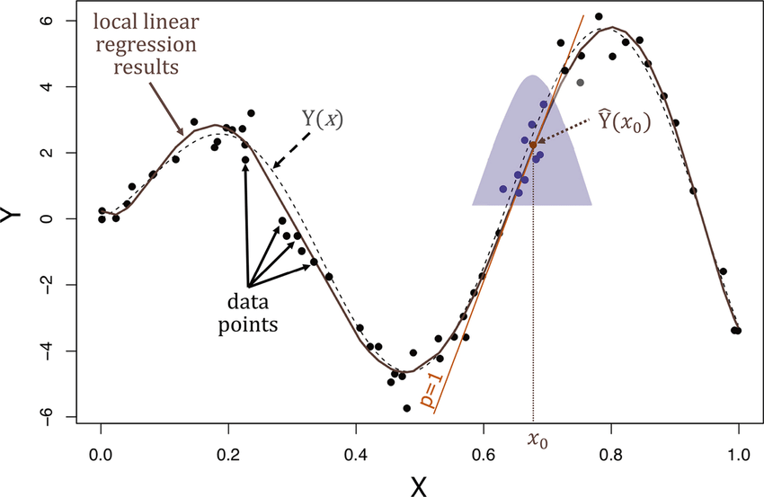
Now, how do you choose the width of this gaussian density? How fat it is? Or how thin should it be? This decides how big a neighborhood should you look in order to decide what’s neighborhood of points you should use to fit this local straight line. And so for gaussian function like this, we use the bandwidth parameter $$ \tau $$, and this is a parameter or hyper-parameter of the algorithm. And depending on the choice of $$ \tau $$, you can choose a fatter or a thinner bell-shaped curve, which causes you to look in a bigger or a narrow window in order to decide how many nearby examples to use in order to fit the straight line.
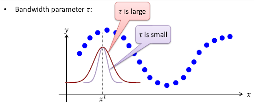
It turns out that, the choice of the bandwidth parameter $$ \tau $$ has an effect on overfitting and underfitting. If $$ \tau $$ is too broad, you end up over-smoothing the data and if $$ \tau $$ is too thin, you end up fitting a very jagged fit to the data.
What happens if you need to infer the value of $$ h $$ outside the scope of the dataset? It turns out that, you can still use this algorithm, it’s just that the results may not be very good. Locally linear regression is usually not greater than exploration, but many learning algorithms are not good at exploration. So all the formulas still work and you can still implement this but the results may not be very good.
We use a locally weighted linear regression when we have a relatively low dimensional dataset. So when the number of features is not too big and we have a lot of data. And you don’t wanna think about what features to use, so that’s the scenario.
It turns out the computation needed to fit the minimization is similar to the normal equations, and so it involves solving a linear system of equations of dimension equal to the number of training examples you have.
Probabilistic Interpretation of Linear Regression
Probabilistic interpretation of linear regression, is a way to interpret linear regression as a probabilistic model.
Why Least Squares? Why Squared Error?
I’m gonna present a set of assumptions, under which these squares using squared error falls out very naturally.
Let’s say for housing price prediction, assume that there’s a true price of every house:
- Where $$ \epsilon^{(i)} $$ is an error term, that includes unmodeled effect and just random noise.
So let’s assume that the way housing prices truly work is that every house’s price is a linear function of the size of the house and number of bedrooms, plus an error term that captures unmodeled effects such as maybe one day that seller is in an unusually good mood or an unusually bad mood, so that makes the price go higher or lower. We just don’t model that as well as random noise.
And we’re going to assume that:
This notation means that $$ \epsilon^{(i)} $$ is distributed Gaussian would mean 0 and covariance $$ \sigma^2 $$.
The $$ N (0, \sigma^2) $$ is a normal distribution also called Gaussian distribution. And what this means is that the probability density of $$ \epsilon^{(i)} $$ is the Gaussian density:
And unlike the bell shaped curve, we used earlier for locally weighter linear regression, this does integrate to 1, and so, this is a Gaussian Density, this is a probability density function.
And this is the familiar gaussian bell shaped curve with mean 0 and covariance $$ \sigma^2 $$, where $$ \sigma $$ kinda control the width of this Gaussian.
 |  |
We assume that the way housing prices are determined is that, first is a true price $$ \theta^T x^{(i)} $$ and then, some random force of nature, the mood of the seller, or any other factors, perturbs it from this true value $$ \theta^T x^{(i)} $$. And the huge assumption we’re gonna make is that the $$ \epsilon^{(i)} $$, these error terms are IID, and IID from statistics stands for Independently and Identically Distributed. And what that means is that, the error term for one house is independent, as the error term for a different house. Which is actually not a true assumption, because if one house is priced on one street is unusually high, then probably a price on a different house on the same street will also be unusually high. But this assumption that these $$ \epsilon^{(i)}\text{s} $$ are IID since they’re independently and identically distributed, is one those assumption that, is probably not absolutely true, but maybe good enough that if you make assumption, you get a pretty good model.
Under these set of assumptions this implies that:
In another way:
Given $$ x^{(i)}; \theta $$, the probability $$ y^{(i)} $$ of a particular house is a Gaussian with mean $$ \theta^T x^{(i)} $$ and variance $$ \sigma^2 $$.
And so because the way that the price of a house is determined, is by taking $$ \theta^Tx $$, the true price of the house, and then adding noise or adding error of variance $$ \sigma^2 $$ to it. and so this assumption imply that given $$ x; \theta $$, the density of $$ y $$, has that distribution, which is $$ y^{(i)} $$ is the random variable, and $$ \theta^Tx^{(i)} $$ is the mean, and $$ \sigma^2 $$ is the variance of the Gaussian density.
The ; in the equation should be read as parameterized by. The alternative way to write that would be to write , instead of ; and this would be conditioning on $$ \theta $$, but $$ \theta $$ is not a random variable, so you shouldn’t condition on it. Which is why we gonna write ; instead.
So, it turns out that, if you are willing to make those assumptions, then linear regression, falls out almost naturally of the assumptions we just made. And in particular, under the assumptions we just made, the likelihood of the parameters $$ \theta $$ which is defined as the probability of the $$ \theta $$ given the data, is:
$$ = \prod_{i=1}^m \mathcal{P}(y^{(i)} \vert x^{(i)}; \theta) $$
And because the error terms are IID to each other, so the probability of all of the observations, of all the values of $$ y $$ in your training set is equal to the product of the probabilities, because of the independence assumption we made.
And so plugging in the definition of $$ \mathcal{P}(y^{(i)} \vert x^{(i)}; \theta) $$, we have:
What’s the difference between likelihood and probability? The likelihood of the parameters, is exactly the same as the probability of the data, but the reason we sometime talk about likelihood and sometimes talk of probability is, the probability of the data is a function of the data as well as a function of the parameters $$ \theta $$, and if you view this number, whatever the number is, and if you view this as a function of the parameters holding the data fixed, then we call that the likelihood. So if you think of the training set the data as a fixed thing, and then varying parameters $$ \theta $$, then we’re going to use the term likelihood. Whereas if you view the parameters $$ \theta $$ as fixed and maybe varying the data, we’re going to say probability. So we can try to say likelihood of the parameters, and probability of the data even though those evaluate to the same thing. For that function, that function is a function of $$ \theta $$ and the parameters, which one are you viewing as fixed and which one are you viewing as variables.
Why $$ \epsilon^{(i)} $$ is Gaussian? It turns out because of central limit theorem, from statistics, most error distributions are Gaussian. If there’s an era that’s made up of lots of little noise sources which are not too correlated, then by central limit theorem it will be Gaussian. So if you think that, most perturbations are, the mood of seller, what’s the school district, what’s the weather like, or access to transportation, and all of these sources are not too correlated, and you add them up then the distribution will be Gaussian.
So you can use the central limit theorem, the Gaussian has become a default noise distribution. But for things where the true noise distribution is very far from Gaussian, thin model do that as well.
We’re going to use lower case $$ \mathscr{l} $$ to denote the log-likelihood.
$$ = \log{\prod_{i=1}^m \frac{1}{\sqrt{2\pi}\sigma} exp({-\frac{(y^{(i)} - \theta^T x^{(i)})^2}{2\sigma^2}})} $$
And as you know, the log of a product is equal to the sum of the logs:
$$ = m \log{\frac1{\sqrt{2 \pi} \sigma}} + \sum_{i=1}^m{-\frac{(y^{(i)} - \theta^T x^{(i)})^2}{2\sigma^2}} $$
One of the well-tested in statistics estimating parameters is to use the maximum likelihood estimation (MLE), which means you choose $$ \theta $$ to maximize the likelihood. So given the dataset, how would you like to estimate the parameters $$ \theta $$? Well, one natural way to choose $$ \theta $$ is to choose whatever value of $$ \theta $$ has a highest likelihood, or in another words, choose a value of $$ \theta $$ so that value, maximizes the probability of the data. And to simplify the algebra, rather than maximizing the likelihood $$ \mathscr{L} $$ is actually easier to maximize the log-likelihood $$ \log{l} $$. But the log is a strictly monotonically increasing function. So the value of $$ \theta $$ that maximizes the log-likelihood should be the same as the value of $$ \theta $$ that maximizes the likelihood.
And if you divide the log-likelihood, we conclude that if you’re using maximum likelihood estimation, what you’d like to do is choose a value of $$ \theta $$ that maximizes this thing.
But the first term, $$ m \log{\frac1{\sqrt{2 \pi} \sigma}} $$, is just a constant, $$ \theta $$ doesn’t even appear in this first term. And what you’d like to do is choose the value of $$ \theta $$ that maximizes the second term:
And so, what you’d like to do is, choose $$ \theta $$ that minimizes this term because of the negative sign:
Because $$ \sigma^2 $$ is just a constant. No matter what $$ \sigma^2 $$ is.
And as you know, this is just $$ \mathcal{J}_\theta $$, the cost function for linear regression.
So, this little proof shows that, choosing the value of $$ \theta $$ to minimize the Least Squares Error, that’s just finding the maximum likelihood estimate for the parameters $$ \theta $$, under this set of assumptions we made, that the error terms as Gaussian and IID.
Is there a situation where using this formula instead of least squares cost function weill be a good idea? No, so this derivation shows that, this is completely to least squares. If you’re willing to assume that the error terms are Gaussian and IID and if you want to use Maximum Likelihood Estimation which is very natural procedure in statistics, than you should use least squares.
If you know for some reason errors are not IID, could you figure out a better cost function? Yes and No. When building algorithms, often we make assumptions about the world that we just know, are not 100% true, because it leads to algorithms that atr computationally efficient. And so, if you knew that your training set was very very non IID, there’re more sophisticated models you could build. But very often we would’t bother, more often than not we might not bother. A few special cases where you would bother there but only if you think the assumption is really really bad, if you don’t have enough data or something quite rare.
So, we set up a set of probabilistic assumptions, we made a certain assumptions about $$ \mathcal{P}(y^{(i)} \vert x^{(i)}; \theta) $$, where the key assumption was Gaussian errors in IID. And then through maximum likelihood estimation, we derived an algorithm which turns out to be exactly the Least Squares algorithm.
Logistic Regression
Logistic regression is a classification algorithm. And what we gonna do is, take that framework, and apply it to the case of classification. And the key steps are:
- Make an assumption about $$ \mathcal{P}(y^{(i)} \vert x^{(i)}; \theta) $$.
- Figure out maximum likelihood estimation.
So, we’re gonna take this framework and apply it to a different type of problem, where the value of $$ y $$ is now either 0 or 1, so is a classification problem.
Binary Classification
A type of classification problem where the value of $y$ is either 0 or 1. So we called it binary classification, because there are only two classes.
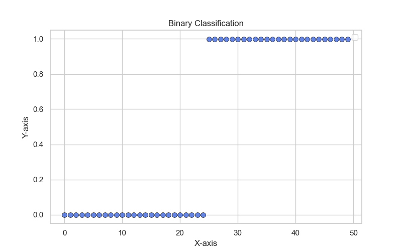
That’s not a good idea to apply linear regression to this dataset. It is tempting to just fit a straight line to this data and then take the straight line and threshold it at 0.5, and then if it’s above 0.5 round off to 1, and if it’s below 0.5 round off to 0.
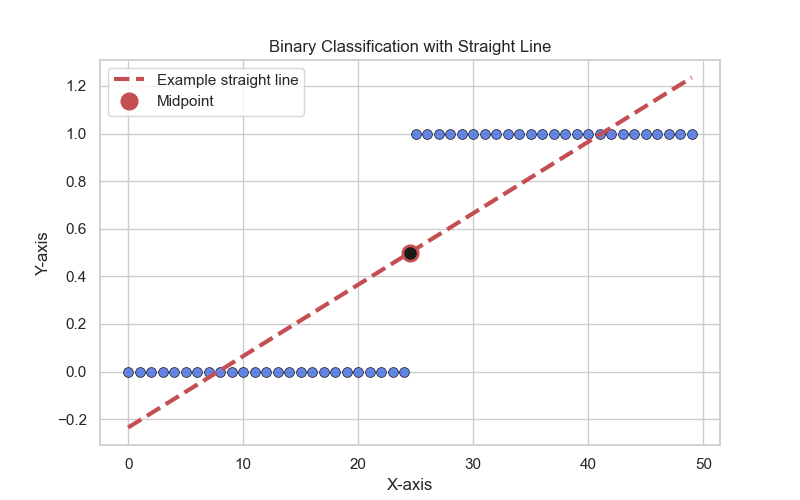
But it turn out that, this is not a good idea for classification problems. And here’s why. Which is for this set it’s really obvious what the pattern is. Everything to the left of the MidPoint predict 0, and everything to the right of that MidPoint predict 1.
But let’s change the dataset to just add one more example as below:
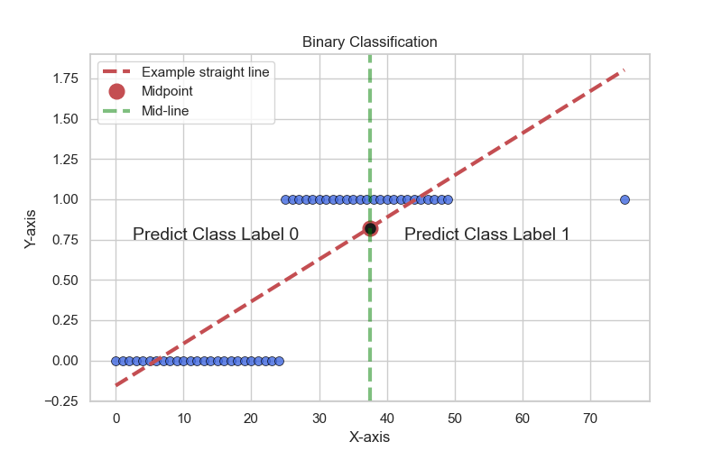
And the pattern still really obvious, but if you fit a straight line to this new dataset with this extra one point, and just not even the outlier, it’s really obvious at this new point way out there should be labeled 1. But with this extra example, if we fit a straight line to the data, as you can see, we end up with a straight line that’s not a good fit, And somehow adding one example, the new straight line is not a good fit. And if you now threshold it at 0.5, you end up with a very different decision boundary.
And so, linear regression is just a good algorithm for classification. And the other unnatural thing about using linear regression for a classification problem is that, you know for a classification problem that the values are 0 or 1, And so it outputs negative values or values even greater than 1 seems strange.
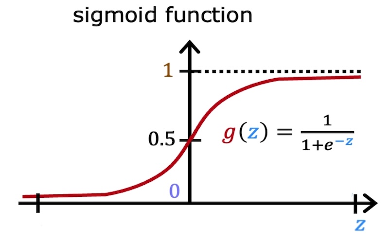
Probably by far the most commonly used classification algorithm is logistic regression. Let’s say the two learning algorithms we probably use the most often are linear regression and logistic regression. So as we designed a logistic regression algorithm, one of the things we might naturally want is for the hypothesis to output values between 0 and 1.
Where the $[0, 1]$ is the set of all numbers from 0 to 1. And so, we’re going to choose the following form of the hypothesis, but first, let’s define the sigmoid function, also called logistic function, which is a function that takes any real number and maps it into the interval $[0, 1]$:
And this function is shaped like as follows, called logistic curve, if you plot this function, you find that it looks like this:
Previously for linear regression we had chosen the hypothesis to be:
We just made a choice that, the housing prices, $h_\theta{(x)}$, are a linear function, $\theta^T x$, of the features $x$. And what logistic regression does is, $\theta^T{(x)}$ could be bigger than 1, or less than 0, which is not very natural. But instead, it’s going to take $\theta^T x$ and pass it through the sigmoid function, so this force the output values only between 0 and 1. So, the hypothesis for logistic regression is:
When designing a learning algorithm, sometimes you just have to choose the form of the hypothesis. How are you gonna represent the function $h$ or $h_\theta$?
And if you’re wondering, there are a lots of functions that we could have chosen and they go between 0 and 1, and why are we choosing this sigmoid function? It turns out that there’s a broader class of algorithms called generalized linear models. And the sigmoid function is a special case of the generalized linear models.
Now, let’s make some assumptions about the distribution of $ y^{(i)} \vert x^{(i)}; \theta $, so we’re going to assume that the data has the following distribution:
From the breast cancer prediction we had, The probability of $y = 1$, it will be the chance of a tumor being cancerous or being malignant, given the size of the tumor, that’s the feature $x$ parameterize by $\theta$, then this is equal to the output of your hypothesis. So in other words, we’re gonna assume that, what you want your learning algorithm to do is, input the features and tell me what’s the chance that this tumor is malignant, what’s the chance that $y = 1$.
And by logic, the chance of $y=0$, has got to be $1-h_\theta{(x)}$. Because if a tumor has a 10% chance of being malignant, that means it has a 90% chance of being benign, since these two probabilities must add up to 1.
Bearing in mind that $y$, by definition, because it is a binary classification problem, can only take on two values, 0 or 1. there’s a nifty sort of little algebra way to take these two equations and write them in one equation. and this will make some of the math a little bit easier.
$$ \mathcal{P}(y \vert x; \theta) = {h_\theta{(x)}}^y {(1 - h_\theta{(x)})}^{1-y} $$
As you can see, because depending on whether $y$ is 0 or 1, one of these two terms switches off, because it’s exponentiated to the power of 0, and anything to the power of 0 is just equal to 1, so one of these terms is just 1.
Now we’re gonna use maximum likelihood estimation again:
$$ = \prod_{i=1}^m \mathcal{P}(y^{(i)} \vert x^{(i)}; \theta) $$
$$ = \prod_{i=1}^m {h_\theta{(x^{(i)})}}^{y^{(i)}} {(1 - h_\theta{(x^{(i)})})}^{1-y^{(i)}} $$
And then, with maximum likelihood estimation, we’ll want to find the value of $\theta$ that maximizes the likelihood of the parameters. And so, same as what we did for linear regression to make the algebra a bit more simple, we’re going to take the log of the likelihood and so compute the log-likelihood.
$$ = \sum_{i=1}^m y^{(i)} \log{h_\theta{(x^{(i)})}} + (1 - y^{(i)}) \log{(1 - h_\theta{(x^{(i)})})} $$
The last thing you want to do is, try to choose the value of $\theta$ to try to maximize $\mathscr{l}(\theta)$.
Batch Gradient Ascent
Is an algorithm to find the maximum of a function.
The differences from what we did for linear regression is the following:
- Instead of $\mathcal{J}(\theta)$, you’re now trying to optimize the log-likelihood instead of this squared cost function.
- Previously you were trying to minimize the squared error,that’s why we had the minus sign, and now you’re trying to maximize the log-likelihood, which is why there’e a plus sign.
So gradient descent is trying to climb down this hill whereas gradient ascent has a concave function like below, and it’s trying to climb up the hill.
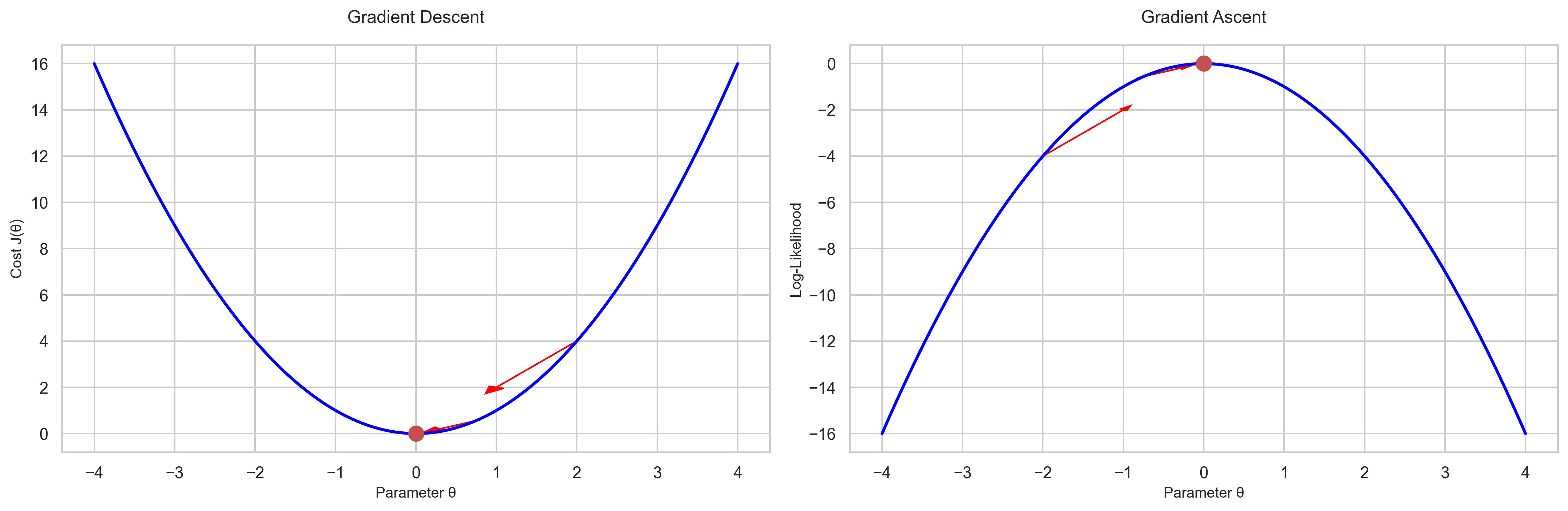
So, that’s why there’s a plus symbol here instead of a minus symbol, because we are trying to maximize the function rather than minimize the function.
If you take derivatives of $\mathscr{l}(\theta)$ with respect to $\theta_j$, so you will find the batch gradient ascent is the following:
Is there a chance of local maximum in this case? No, there isn’t. It turns out that this function, the log-likelihood function $\mathscr{l}(\theta)$, full logistic regression, it always looks like the plot we saw above. So this is a concave function, and there are no local optimum, the only maximum is a global maximum. There’s actually another reason why we chose the logistic function, because if you choose a logistic function rather than some other function that will give you 0 to 1, you guaranteed that the likelihood function has only one global maximum.
Is there a equivalent of normal equations for logistic regression? Short answer is no. So for linear regression the normal equations gives you like a one shot way to just find the best value of $\theta$. There is no known way to just have a close form equation, unless you find the best value of $\theta$ which is you always have to use an algorithm, an iterative optimization algorithm such as Gradient Ascent and Newton’s Method.
Newton’s Method
Newton’s method is a way to find the roots of a function. Which is used in logistic regression.
Gradient ascent is a good algorithm, we use gradient ascent all the time, but it takes a much baby steps, it takes a lot of iterations for gradient ascent to converge. There’s another algorithm called Newton’s Method, which allows you to take much bigger jumps. There are problems where you might need 100 or 1000 iterations of gradient ascent, that if you run newton’s method algorithm, you might need only 10 iteration to get a very good value of $\theta$. But each iteration will be more expensive.
Let’s describe this algorithm, which is sometimes much faster than gradient ascent for optimizing the value of $\theta$. So let’s use this simplified one-dimensional problem to describe Newton’s method. We’re gonna to solve a sightly different problem with Newton’s method, which is say you have some function $f$, and you want to find a $\theta$ such that $f(\theta) = 0$. So this is a problem that Newton’s method solves. And the way we’re gonna to use this late is, what you really want is to maximize $\mathscr{l}_\theta$, and well at the maximum, the first derivative, must be 0. I.e. you want to value, where the derivative $\mathscr{l}’ (\theta) = 0$. And $\mathscr{l}’$ is the derivative of $\theta$ because this is where $\mathscr{l}’$ is another notation for the first derivative of $\theta$.
So, you want to maximize or minimize a function, what that really means is, you want to find a point where the derivative is equal to 0. So the way we’re going to use Newton’s method is, we’re going to set $f(\theta)$ equal to the derivative, $\mathscr{l}’$, and then try the point where the derivative is equal to 0.
But to explain Newton’s method, we’re gonna work on this other problem where you have a function $f$ and you just want to find a value of $\theta$ where $f(\theta) = 0$, And we’ll set $f$ equal to $\mathscr{l}’(\theta)$, and that’s how we’ll apply this to logistic regression.
So let’s break down the algorithm based on the plot below:
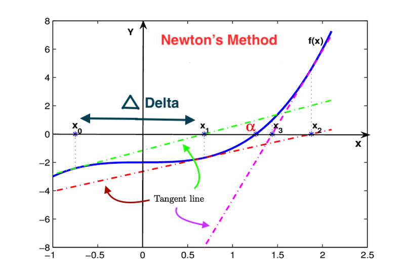
So, let’s say function $f$ which has blue color, and the goal is to find the value of $\theta$ where $f(\theta) = 0$, which in this example is called $\alpha$. So, let’s say you start off at $x_0$ point at the first iteration, you have randomly initialized data, and actually $\theta$ is 0 or something, this is how one iteration of Newton’s method will works. What we’re going to do is look at the function $f$, and then find a line that is just tangent to $f$. So take the derivative of $f$ and find a line that is just tangent to $f$. And we’re gonna use a straight line approximation to $f$, and solve for where $f$ touches the horizontal axis. So we’re gonna solve for the point where the green straight line touches the horizontal axis, which is $x_1$. And that’s one iteration of Newton’s method, so we’re gonna move from $x_0$ to $x_1$. And then in the second iteration of Newton’s method, repeat these steps for the $x_1$ point, and so on.
So you can tell that, Newton’s method is actually a pretty fast algorithm. When in just 3 or 4 iterations, we’ve gotten really close to the point where $f(\theta) = 0$.
Let’s write out the math for how you do this. So, let’s just write out the derive, how you go from $x_0$ to $x_1$. So what we’d love to do is solve for the value of $\Delta$, distance between $x_0$ and $x_1$. Because one iteration of Newton’s method is:
$$ f'(\theta^{(0)}) = \frac{f(\theta^{(0)})}{\Delta} $$
$$ \Delta = \frac{f(\theta^{(0)})}{f'(\theta^{(0)})} $$
And you plug in $\Delta$ into $\theta^{(i)} := \theta^{(0)} - \Delta$, then you find that a single iteration of Newton’s method is the following:
Note that here, $\theta$ is the $x$ in the plot above.
And finally:
Because we wanna find the place where the first derivative of $\mathscr{l}$ is equal to 0. So:
So it’s really the first derivative divided by the second derivative.
Newton’s method is a very fast algorithm, and enjoys a property called Quadratic Convergence. In formally, what it means is that, if on one iteration Newton’s method has 0.01 error, so on the $x$ axis, you’re 0.01 away from the true minimum, or the tru value of $f$ is equal to 0. After one iteration, the error could go to 0.0001 error, and after two iterations it goes 0.00000001 error. But roughly Newton’s method, under certain assumptions, that function move not too far from quadratic, the number of significant digits that you have, converged the minimum doubles on a single iteration. So this called Quadratic Convergence. And so when you get near the minimum, Newton’s method converges extremely rapidly. So after a single iteration, it becomes much more accurate, and after another iteration, it becomes much more accurate. Which is why Newton’s method required relatively few iterations.
We have seen the Newton’s method for when $\theta$ is a real number, when $\theta$ is a vector, than the generalization of the rule, which we seen above, is the following:
- Where $H$ is the Hessian matrix, which is the matrix of second derivatives.
- $\nabla_\theta \mathscr{l}$ is the vector of derivatives. and has $\mathbb{R}^{n+1}$ dimensions, if $\theta\in{\mathbb R^{n+1}}$. Then this derivative respect to the $\theta$ of the log-likelihood becomes a vector of derivatives. And the Hessian matrix, becomes a matrix as $\mathbb{R}^{(n+1)\times({n+1})}$. So it becomes a squared matrix with the dimension equal to the parameter vector $\theta$.
And the Hessian matrix is defined as the matrix of partial derivatives.
The disadvantage of Newton’s matrix is that, in high-dimensional problems, if $\theta$ is a vector, than each step of Newton’s method is much more expensive, because you’re either solving a linear system equations, or having to invert a pretty big matrix. So if $\theta$ is ten-dimensional, this involves inverting a 10 by 10 matrix, which is fine, but if $\theta$ was 10,000 or 100,000, then each iteration requires computing like a 100,000 by 100,000 matrix and inverting that, which is very hard. It’s actually very difficult to do that in very high-dimensional problems.
Some rules of thumb:
- If the number of parameters in your iteration is not too big, if you have 10 or 50 parameters, you would very likely use Newton’s method. Because then you probably get convergence in maybe 10 or 15 iterations or even less than 10 iterations.
- But if you have a very large number of parameters, if you have 10,000 parameters, then rather than dealing with a 10,000 by 10,000 matrix, or even bigger, the 50,000 by 50,000 matrix and you have 50,000 parameters, you would use gradient descent.
- But if the number of parameters is not too big, so that the computational cost per iteration is manageable, then Newton’s method converges in a very small number of iterations, and could be much faster algorithm than gradient ascent.