Linear Regression
Definition
Linear Regression is one of the simplest supervised learning algorithms, which is used to predict a continuous value.
You can see the ALVINN video, the autonomous driving video, for the self-driving car, in the previous post Introduction to Machine Learning, that was a supervised learning problem. And that was a Regression problem, because the output Y that you want is a continuous value.
Rather than using a self-driving car example which is quite complicated, let’s build up a supervised learning algorithm using a simpler example.
Designing a Learning Algorithm
House Price Prediction Example:
Let’s say you want to predict or estimate the prices of houses. So the way you should building a learning algorithm is start by collecting dataset of houses and their prices.
Here is the sample data of house size and price:
| Size ($$ feet^2 $$ ) | Price ($1Ks) |
|---|---|
| 2104 | 400 |
| 1416 | 232 |
| 1534 | 315 |
| 852 | 178 |
The process of supervised learning is that you have a training set such as the dataset that we have above, and you feed this to a learning algorithm, and the job of the learning algorithm is to output a function to make predictions about housing prices. And by convention, we gonna call this a function that it outputs a hypothesis, and the job of the hypothesis is, it can take input the size of a new house, that you haven’t seen yet, and will output the estimated price.
Here is the Linear Regression learning algorithm:
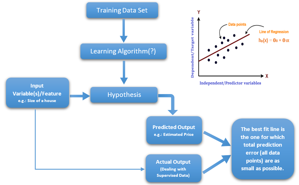
So the job of the learning algorithm is to input a training set, and output a hypothesis. The job of the hypothesis is to take as input, any size of a house in this example, and try to tell you what it thinks should be the price of that house.
When designing a learning algorithm, even through linear regression, you may have seen it in a linear algebra, the eay you go about structuring a machine learning algorithm is important. And design choices of, what is the workflow? What is the dataset? What is the hypothesis? How does this represent the hypothesis? These are the key decisions you have to make in pretty much every supervised learning, every machine learning algorithm’s design.
These concepts will lay the foundation for the rest of the algorithms.
Hypothesis Representation
As a emerging discipline grows up, notation kind of emerges depending on what different scientists use for the first time when you write a paper. I think that the fact that we call these things hypothesis, frankly, i don’t think that’s a great name. But i think someone many decades ago wrote a few papers calling it a hypothesis, and then others fallowed, and we’re kind of stuck with some of this terminology. 1
So, when designing a learning algorithm, the first thing we need to ask is, how do you represent the hypothesis h? And in linear regression, we’re going to say that:
That shows the input size X and output a number as a linear function of the size X.
Technically this is an affine function. It was a linear function, there’s no $$ \theta_0 $$, technically, but in machine learning sometimes just calls this a linear function.
In this example we have just one input feature X. More generally, if you have multiple input features, such as table below:
| Size ($$ feet^2 $$ ) | Number of Bedrooms | Price ($1Ks) |
|---|---|---|
| 2104 | 3 | 400 |
| 1416 | 2 | 232 |
| 1534 | 3 | 315 |
| 852 | 2 | 178 |
So, more generally, if you know the size of the house, as well as the number of bedrooms in these houses, then you may have two input features, where $$ X_1 $$ is the size, and $$ X_2 $$ is the number of bedrooms, here is how you can represent the hypothesis:
So in order to simplify the notation, and make that a little bit more compact, I’m gonna introduce this other notation:
So this is the summation, where for conciseness we define $$ X_0 $$ to be equal to 1.
Here $$ \theta $$ becomes a three-dimensional parameter: $$ \theta_0 $$, $$ \theta_1 $$, and $$ \theta_2 $$. This index starting from 0, and the features become a three-dimensional feature vector: $$ X_0 $$, $$ X_1 $$, and $$ X_2 $$, where $$ X_0 $$ is always 1, $$ X_1 $$ is the size of the house, and $$ X_2 $$ is the number of bedrooms.
So, to introduce a bit more terminology, $$ \theta $$ is called the parameters of the learning algorithm, and the job of the learning algorithm is to choose parameters $$ \theta $$ that allows you to make good predictions about your prices of houses.
Just to lay out some more notation, We’re gonna use a standard, $$ m $$, we’ll define as the number of training examples, so $$ m $$ is going to be the number of rows. Where each house you have in your training set is a training example.
And already seen, we use $$ X $$ to denote the inputs, and often the inputs are called features and input features or sometimes input attributes.
And, $$ y $$, is the output, and sometimes we call this the target variable or label.
And so, $$ (x, y) $$ is one training example:
And, we going to use $$ n $$ to denote the number of features you have for the supervised learning problem. SO in this example, $$ n $$ is equal to 2, because we have two features which are the size of house and the number of bedrooms.
So, we can write the hypothesis as:
And so here, $$ X $$ and $$ \theta $$ are $$ n+1 $$ dimensional, because we added the extra $$ x_0 $$ and $$ \theta_0 $$, so we have two features in the house price prediction example, then these are three-dimensional vectors.
And $$ x_0 $$ is always equal to 1.
Cost Function
The learning algorithm’s job is to choose values for the parameters $$ \theta $$, so that it can output a hypothesis. So how do you choose parameters $$ \theta $$?
Well, what we’ll do, is let’s choose $$ \theta $$ such that $$ h(x) $$ is close to $$ y $$ for the training examples.
The final bit of notation, I’ve been writing $$ h(x) $$ as a function of the features of the house, as a function of the size and number of bedrooms of the house, sometimes we emphasize that $$ h $$ depends both on the parameters $$ \theta $$ and on the input features $$ X $$.
Sometimes for notational convenience, we just write this as $$ h(x) $$, and sometimes we include the $$ \theta $$ parameter and write as $$ h_{\theta}(x) $$, and they mean the same thing, it’s just maybe a abbreviation in notation.
So, in order to learn a set of parameters, what we’ll want to do is choose a parameters $$ \theta $$, so that at least for the house whose prices you know, the learning algorithm outputs prices that are close to what you know where the correct price is for that set of houses.
And so formally, in the linear regression algorithm, also called Ordinary Least Squares, we will want to minimize the square difference between what the hypothesis outputs (prediction), and $$ y $$ which is the correct price, by choosing the values of $$ \theta $$.
To fill this out, you have $$ m $$ training examples , so we going to sum from $$ i = 1 $$ through $$ m $$ of that square difference. So, this is sum over all the $$ m $$ training examples.
Finally, by the convention, we put a one-half constant there, because when we take derivatives to minimize this later, putting a one-half there would make some of the math a little bit simpler. Minimizing that formula should give you the same as minimizing one-half of that.
In Linear Regression we’re gonna define the Cost Function as below:
And we’ll find parameters $$ \theta $$ that minimizes the cost function $$ J_{\theta} $$.
Gradient Descent
Definition
Now, we need to implement an algorithm to find the value of $$ \theta $$ that minimizes the cost function $$ J_{\theta} $$.
We’re going to use an algorithm called Gradient Descent. With gradient descent we are going to start with some value of $$ \theta $$, and it could be $$ \theta $$ equals the vector of all zeros would be a reasonable default, we can initialize it randomly, the count doesn’t really matter.
This was initial value of $$ \theta $$, and we’re going to keep changing that to reduce the cost function, $$ J_{\theta} $$.
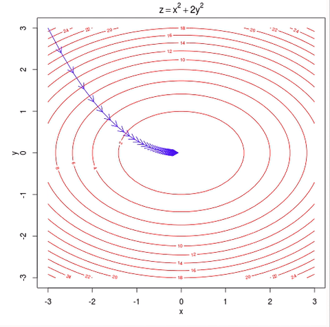
Visualization of Gradient Descent
As the plot below shows, what you want to do is find values for $$ \theta_0 $$ and $$ \theta_1 $$, that minimize the height of the surface, $$ J_{\theta} $$.
note that in house price prediction example we have 3 parameters, but we can plot that, so we just using 2 parameters in this example for simplicity.
And so, in gradient descent you start off at some point on this surface and you do that by initializing $$ \theta_0 $$ and $$ \theta_1 $$ either randomly or to the value of all zeros or something, it doesn’t matter too much.
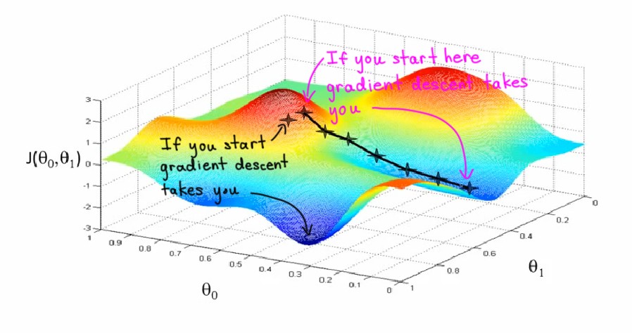
Imagine that you standing on some random point on this surface, what you do in gradient descent is, turn around all 360 degrees and look all around you, and see if you were to take a tiny little step, in what direction should you take that little step, to go downhill as fast as possible. Because you’re trying to go downhill which is goes to the lowest possible elevation, lowest possible point of $$ J_{\theta} $$, because you want to minimize and reduce the value of $$ J_{\theta} $$
So, gradient descent will take that little baby step, and then repeat and repeat until hopefully, you get to a local optimum.
One property of gradient descent is that, depend on where you initialize parameters, you can get to a different local optimum and minimum, as you can see in the plot above.
Formalize Gradient Descent Algorithm
In gradient descent, each step of the algorithm is implemented as follow, just remember in this example, the training set (dataset) is fixed, and the cost function $$ J_{\theta} $$ is a fixed function, there’s function of parameters $$ \theta $$, and the only thing you’re gonna do is tweak or modify the parameters $$ \theta $$.
So, a bit more notation, we’re gonna use $$ := $$ to denote assignment, so what this means is, we’re gonna take the value on the right and assign it to the variable on the left, for example, $$ a := a+1 $$ means that increment the value of $$ a $$ by $$ 1 $$.
And the $$ a=b $$ is asserting a statement of fact, asserting that the value of $$ a $$ is equal to the value of $$ b $$.
So, in each step of gradient descent, you’re going to for each value of $$ j $$, you’re going to update $$ \theta_j $$ as follows:
Where the $$ \alpha $$ is the learning rate, and $$ \frac{\partial}{\partial \theta_j} J(\theta) $$ is the partial derivative of the cost function $$ J(\theta) $$ with respect to the parameter $$ \theta_j $$.
You may know that the derivative of a function is, defines the direction of steepest descent. So it defines the direction that allows you to go downhill as steeply as possible.
Now, let’s see just quickly how the derivative calculation is done:
$$ = 2 * \frac{1}{2} (h_{\theta}(x) - y) * \frac{\partial}{\partial \theta_j} (h_{\theta}(x) - y) $$
$$ = (h_{\theta}(x) - y) * \frac{\partial}{\partial \theta_j} (\theta_0 x_0 + \theta_1 x_1 + ... + \theta_n x_n - y) $$
$$ = (h_{\theta}(x) - y) * x_j $$
So plugging it back into that formula, one step of gradient descent is the following:
Note that we did this with one training example, we kind of used definition of the cost function $$ J_{\theta} $$ defined just one single training example, but you actually have $$ m $$ training examples. So the correct formula of the derivative is actually if you take the result of partial derivation and sum it over all $$ m $$ training examples, we get the correct formula for partial derivative as follows:
So, base on that the gradient descent algorithm is:
Note that, the derivative of a sum is the sum of derivatives.
And so, the gradient descent algorithm is to repeat until convergence, carry out this update, and in each iteration of gradient descent, you do this update for $$ j = 0 $$ through $$ n $$, where $$ n $$ is the number of features.
If you do this then, what will happen is you find a pretty good value of the parameters $$ \theta $$.
It turns out that, when you plot the cost function $$ J_{\theta} $$ for a linear regression model, unlike the earlier diagram we saw, which has local optimum, it turns out that if $$ J_{\theta} $$ is defined the way we just defined it for linear regression, is the sum of square terms, then $$ J_{\theta} $$ turns out to be a quadratic function. It’s a sum of these squares of terms, and so $$ J_{\theta} $$ will always look like a big bowl like the plot below, and so $$ J_{\theta} $$ does not have the local optimum, or the only local optimum is also the global optimum.
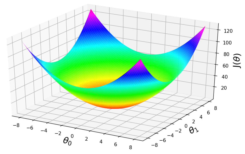
The other way to look at the function like this is to look at the contours of this plot. So you plot the contours by looking at the big bowl, and taking horizontal slices and plotting where the edges of the horizontal slice is. So the contours of a big bowl or of this quadratic function will be ellipsis.
And if you run gradient descent on this algorithm, then with each step of gradient descent, the algorithm will take that step downhill, because there’s only one global minimum, this algorithm will eventually converge to the global minimum.
Fun fact, if you thinking about the contours of the function, it turns out the direction of the steepest descent is always at 90 degrees, is always orthogonal to the contour direction.
Now let’s see how we should choose the Learning Rate $$ \alpha $$. If you set $$ \alpha $$ to be very very large, to be too large then they can overshoot, the steps you take can be too large and you can run past the minimum, and if you set to be too small, then you need a lot of iterations and the algorithm will be slow.
And so what happens in practice is, usually you try a few values and see what value of learning rate allows you to most efficiently drive down the value of $$ J_{\theta} $$. And if you see the cost function $$ J_{\theta} $$ increasing rather than decreasing, then there’s a very strong sign that the learning rate is too large.
And what we should often do is to try out multiple values of the learning rate $$ \alpha $$ and usually try them on an exponential scale, so you try 0.01, 0.02, 0.04, 0.08, … kinda like a doubling scale or tripling scale and try a few values and see what value allows you to drive down to the learning rate fastest.
If you had question about why we are subtracting learning rate $$ \alpha $$ times the gradient rather than adding it, i’m going to say that the reason is that we want to move in the opposite direction of the gradient as you can see in the plots above, to minimize the cost function $$ J_{\theta} $$.
Batch Gradient Descent
Gradient descent and linear regression is definitely still one of the most widely used learning algorithms in the world today. And if you implement this, you could use this for some actually pretty decent purposes.
Gradient descent algorithm, calculates this derivative by summing over your entire training set, and sometimes this version of gradient descent has another name, which is called Batch Gradient Descent.
I think in Machine Learning, our whole committee, we just make up names and stuffs and sometimes the names aren’t great. 1
The term Batch Gradient Descent refers to that, you look at the entire training set, you think of all examples in the training set as one batch of data, and you’re going to process all the data as a batch, so hence the name Batch Gradient Descent.
The disadvantage of batch gradient descent is that if you have a giant dataset, such as in era of big data which we’re really moving to larger and larger datasets, in order to make one update to your parameters, in order to even take a single step of gradient descent, you need to calculate that sum over all training examples, and if $$ m $$ is a million or 100 million, you need to scan through entire dataset. And so every single step of gradient descent becomes very slow and expensive.
So, if you have a large dataset, you might want to use a different version of gradient descent, which is called Stochastic Gradient Descent.
Stochastic Gradient Descent
There’s an alternative to batch gradient descent, which is called Stochastic Gradient Descent.
This algorithm, instead of scanning through all million examples before you update the parameters $$ \theta_j $$ even a little bit, instead, in the inner loop of the algorithm, loop through $$ i=1 $$ through $$ m $$ of taking a gradient descent step, using the derivative of just one single example, update $$ \theta_j $$ using the derivative we just calculated with respect to one training example and update that for every $$ j $$.
As you run stochastic gradient descent, it takes a slightly noisy, random path toward the minimum, but on average, it’s headed toward the global minimum.
Stochastic gradient descent will actually never converge, but in batch gradient descent, it kind of went to the global minimum and stopped. But with stochastic gradient descent, the parameters will oscillate and won’t ever quite converge because you’re always running around looking at a different random example and trying to do better than just that one example. But when you have a very large dataset, stochastic gradient descent allows your implementation and algorithm to make much faster progress, and it is used much more, in practice, than batch gradient descent.
In practice, we can slowly decrease the learning rate, so just keep using stochastic gradient descent, but reduce the learning rate over time, so it takes smaller and smaller steps. If you do that, then what happens is the size of the oscillations would decrease, and so you end up oscillating or bouncing around the smaller region. So wherever you end up, may not be the global global minimum, but at least it will be closer to the global minimum.
We can use plot to $$ J_{\theta} $$ over time, so $$ J_{\theta} $$ is the cost function that you’re trying to drag down, so monitor $$ J_{\theta} $$ and it is going down over time, and then if it looks like it stopped going down we can stop training.
One nice thing about linear regression is that it has no local optimum and so, you run into there convergence debugging types of issues less often. When you training highly non-linear things like neural networks, these issues become more acute.
If you have a relatively small dataset, it’s computationally efficient to do batch gradient descent, if batch gradient descent doesn’t cost too much, because it’s one less thing to fiddle with and worry about, like the parameters oscillating, but if your dataset is too large that batch gradient descent becomes prohibitively slow, than you should use stochastic gradient descent or whatever more like that.
Normal Equation
Gradient descent, both batch gradient descent and stochastic gradient descent, is an iterative algorithm meaning that you have to take multiple steps to hopefully, get near the global optimum. It turns out there is another algorithm, for the special case of linear regression, and it turns out there’s a way to solve for the optimal value of the parameters $$ \theta $$ to just jump in one step to the global optimum without needing to use an iterative algorithm.
This algorithm is called Normal Equation and it works only for linear regression.
We are going to use the following notation, called as matrix derivative notation that allows you to derive the normal equation in roughly four lines of linear algebra, rather than some pages and pages of linear algebra and in the Machine Learning sometimes notation really matters, if you have right notation you can solve some problems much more easily.
So, let’s define this Matrix Linear Algebra notation, and then we don’t wanna do all the steps of derivation, we gave the sense of the flavor of what it look like. this notation is really convenient for deriving learning algorithms.
Where:
- $$ J_{\theta} $$ : There’s a function mapping from parameters to the real numbers.
- $$ \nabla_{\theta} J(\theta) $$ : This is the derivative of $$ J_{\theta} $$ with respect to $$ \theta $$.
- $$ {\theta} \in{\mathbb{R}}^{(n+1)} $$ : $$ \theta $$ is a n+1 dimensional vector.
Example: Let’s say that $$ A $$ is a two-by-two matrix.
Then you might have some function of a matrix $$ A $$, then that’s a real number.
$$ f({\begin{bmatrix} 3 & 4 \\ 5 & 6 \end{bmatrix}}) = 3 + 4^2 = 19 $$
So, as we derive this, this is an example of a function that inputs a matrix and maps the values of matrix to a real number. And when you have a matrix function like this, we will going to define the derivative with respect to $$ A $$ of $$ f(A) $$ as follows:
So if $$ A $$ was a 2-by-2 matrix then $$ \nabla_A f(A) $$ is itself a 2-by-2 matrix, and you compute this matrix just by looking at $$ f(A) $$ and taking derivatives with respect to each of the elements and plugging them into the matrix.
And so in that particular example:
So, that’s the definition of a matrix derivative. And now, you know well, how do you minimize a function? you take derivatives with respect to $$ \theta $$ and set it equal to zero, and then you solve for the value of $$ \theta $$ so that the derivative is 0. The maximum and minimum of a function is where the derivatives is equal to 0. So, how you derive the normal equation is take this vector, so $$ J_\theta $$ maps from a vector to a real number. So we’ll take the derivatives respect to $$ \theta $$ ans set it to 0 and solve for $$ \theta $$ and then we end up with a formula for $$ \theta $$ that lets you just immediately go to the global minimum of the cost function $$ J_\theta $$.
Now, just a couple other derivations.
If $$ A \in{\mathbb{R}}^{(n*n)} $$ is a square matrix, we’re going to denote the trace of $$ A $$ to be equal to the sum of the diagonal entries.
You can also write this as trace operator $$ tr(A) $$ like the trace function applied to $$ A $$, but by convention we often write $$ trace A $$ without the parentheses. So trace just means sum of diagonal entries.
Some fact about the trace of a matrix:
- $$ tr A = tr A^T $$
Because if you transpose a matrix, you’re just flipping it along the 45 degree axis, and so the diagonal entries actually stay the same when you transpose the matrix. - $$ f(A) = tr AB $$
So here is $$ B $$ is some fixed matrix, and what $$ f(A) $$ does is it multiplies $$ A $$ and $$ B $$ and then it takes the sum of diagonal entries. Then it turns out that:
$$ \nabla_A f(A) = B^T $$ - $$ tr AB = tr BA $$
- $$ tr ABC = tr CAB $$
This is a cyclic permutation property, if you have a multiply several matrices together you can always take one from the end and move it to the front and the trace will remain the same. - $$ \nabla_A tr AA^TC = CA + C^TA $$
Think of this as analogous to $$ \frac{\partial}{\partial a} a^2c = 2ac $$ but that is like the matrix version of that.
So finally, we’re going to take $$ J_{\theta} $$ and express it in this matrix vector notation. So we can take the derivatives with respect to $$ \theta $$ and set it equal to 0 and solve for value of $$ \theta $$.
And if you define matrix capital $$ X $$ as follows:
We call this the design matrix. and it turns out that if you define $$ X $$ this way, then:
And the way a matrix vector multiplication works is you multiply the column vector $$ \theta $$ with each of those rows of $$ X $$. And so this ends up being a column vector, which is:
Which is of course just the vector of all the prediction of the algorithm as you can see. Now let also define a vector $$ y $$ to be taking all of the labels from your training examples, and stacking them up into a big column vector.
It turns out that:
If we wanna proof that:
So, it’s just all the error your learning algorithm is making on the $$ m $$ examples. It’s difference between predictions and the actual labels.
And as you know, a vector transpose multiplied by itself is equals to the sum of squares of elements. So:
So that’s why you end up with this:
Now what we wanna do is take the $$ \nabla_{\theta} J(\theta) $$ and set it equal to 0. So:
$$ = \frac12 \nabla_{\theta} {(\theta^T x^T - y^T)} (x \theta - y) $$
$$ = \frac12 \nabla_{\theta} [\theta^T x^T x \theta - \theta^T x^T y - y^T x \theta + y^T y ] $$
What we just did here, this is similar to this:
It’s just expanding out a quadratic function.
And then the final step is for each of those four terms, to take the derivative with respect to $$ \theta $$. And at the end you find that the derivative is:
$$ = x^T x \theta - x^T y = \overrightarrow{0} $$
$$ x^T x \theta = x^T y $$
And finally, this is called the Normal Equation. And the optimum value for $$ \theta $$ is:
And if you implement this, than you can in basically one step, get the value of that corresponds to the global minimum.
And a common question is, what if $$ X^T X $$ is not invertible? what that usually means is you have redundant features. That your features are linearly dependent. But if you use something called the Pseudo-Inverse, you kind of get the right answer if that’s the case. Although, if you have linearly dependent features, probably means you have the same feature repeated twice, and you should go and figure out what features are actually repeated, and leading to this problem.